


ICB User information
Area coverage
Table 1.1, Table 1.2 and Figure 1.1 provide an overview of the area of coverage for dryland and irrigated summer crops in South Africa’s key agro-ecological producing regions. The coordinators of this initiative are sincerely grateful for the interaction and assistance with data, knowledge and other inputs from each organisation, agribusiness and farmers.
| Area | Dryland crops | Source and Collaborators |
|---|---|---|
| KwaZulu-Natal | ||
| Bloedrivier | Maize and soybeans | GSA, Senwes and BFAP |
| Mpumalanga | ||
| Middelburg / Trichardt | Maize, soybeans and grain sorghum | GSA, Senwes and BFAP |
| Ermelo | Maize and soybeans | GSA, Senwes and BFAP |
| Eastern Free State | ||
| Reitz region | Maize, soybeans, sunflower and dry beans | GSA, VKB, Senwes and BFAP |
| Northern Free State | ||
| Northern Free State – water table soils / higher potential | Maize | GSA, Senwes and BFAP |
| Northern Free State – normal potential | Maize | GSA, Senwes and BFAP |
| Northern Free State | Maize, soybeans, sunflower, groundnuts and grain sorghum | GSA, Senwes and BFAP |
| North West | ||
| Koster | Maize, soybeans and sunflower | GSA, NWK, Senwes and BFAP |
| Lichtenburg | Maize, soybeans, sunflower and groundnuts | GSA, NWK, Senwes and BFAP |
| Area | Irrigated crops | Source and Collaborators |
|---|---|---|
| Northern Cape | ||
| GWK area | Maize, soybeans, groundnuts and sunflower | GWK, GSA and BFAP |
| KwaZulu-Natal | ||
| Bergville | Maize and soybeans | GSA and Senwes |
| North West | ||
| Britz / Northam / Koedoeskop | Maize, soybeans, sunflower and sorghum | GSA and NWK |
| Limpopo | ||
| Loskop Irrigation Scheme | Maize and soybeans | GSA and Senwes |

Model Assumptions
The Bureau for Food and Agricultural Policy (BFAP) annually provides a baseline outlook on agricultural production, consumption, prices, and trade in South Africa over a 10-year horizon. This outlook is developed using the BFAP system of models and is grounded in a coherent set of assumptions regarding a range of economic, technological, environmental, political, institutional, and social factors. Among these critical assumptions, one of the most significant is the expectation that stable weather conditions will prevail in Southern Africa and globally, allowing for consistent yield growth as technology advances. Therefore, the outlook is not a forecast but rather a plausible future scenario based on fundamental market drivers. It serves as a projection of a potential future equilibrium, providing a benchmark against which further analyses can be evaluated.
The assumptions regarding the future macroeconomic environment are based on a combination of projections from the International Monetary Fund (IMF), the World Bank, and the Bureau for Economic Research (BER) at Stellenbosch University. Baseline projections for global commodity markets are sourced from the Food and Agricultural Policy Research Institute (FAPRI) at the University of Missouri and the Food and Agriculture Organization (FAO) of the United Nations. Once these assumptions are integrated into the BFAP system of models, the outlook for all commodities is simulated within a closed system of equations. This process captures the interconnections between sectors—so that, for instance, shocks in the grain sector are transmitted to the livestock sector, and vice versa. For each commodity, key components of supply and demand are identified, and equilibrium is established through balance sheet principles, ensuring that total demand equals total supply.
Yield assumptions
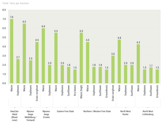
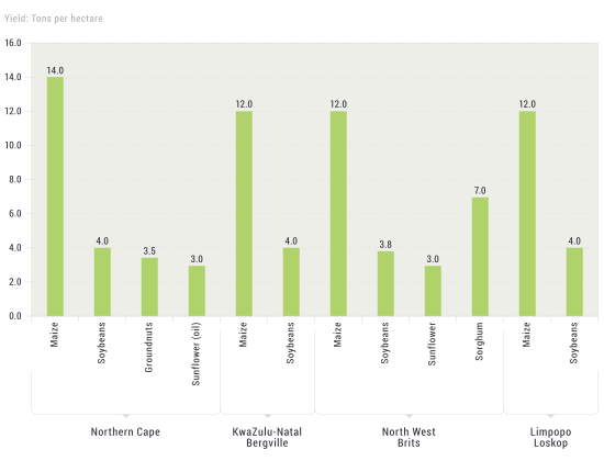
Figure 1.1 and Figure 1.2 indicate the yield assumptions for dryland and irrigated crops. These assumptions represent target yields which were formulated in round table discussions. These levels are based on crop potential in the respective regions, historic trends and expert opinions. It is important to note that intra-regional variations will occur, and it is recommended that producers adjust their target yields based on their location and potential.
Crop price assumptions
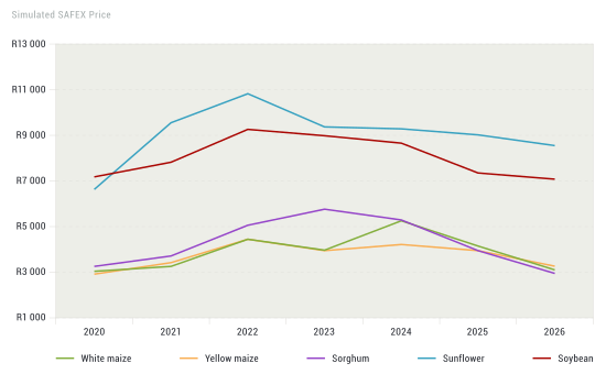
Figure 1.3 illustrates the key commodity price assumptions for white maize and yellow maize, sorghum, sunflower and soybeans that were used in the summer crop budgets for the 2025/26 production season. Further deductions were made to calculate a farm gate price for each agro-ecological producing region. The sensitivity analysis in the respective crop budgets makes provision for variation in price and yield and indicates the gross margin under each price and yield combination.
Global crop prices have stabilised after an initial drop, but the medium-term trend remains downward in real terms. South African prices lag due to the 2024 drought, even though sharp declines occurred in between August and September 2025. On 30 September, South Africa’s Crop Estimates Committee released its 8th forecast, revising maize production up from 15.80m to 16.18m tons — a 2.4% increase (376,200 tons). Soybean and sunflower output remain largely unchanged (CEC, 2025).
After reaching a peak in 2022, global commodity prices have generally declined, with the notable exception of sunflower, which experienced an increase between August 2024 and April 2025 (Grain SA, 2025). Since June, the price of global yellow maize (US) dropped below $200 per ton, trading at $183 per ton, marking a 48% decrease from its peak in the second quarter of 2022. Wheat, soybeans, and sunflower have followed similar downward trajectories (FAO, 2025). Domestically, a stronger Rand and a robust 2025 summer crop contributed to sharp price reductions in September. Compared to January 2025, yellow maize fell by 36%, soybeans by 24%, while sunflower and wheat saw modest increases of around 4%. Despite these recent declines, prices remain significantly higher than in 2019, with yellow maize, soybeans, and wheat being approximately 36% higher, and sunflower prices have nearly doubled. A strong 2026 harvest could bring maize prices closer to export parity.
Source: BFAP, November 2025
Key input cost trends
Figure 1.4 illustrates the cost trends for fuel and fertilisers over the period from January 2022 to August 2025. Agricultural input costs remain high and volatile, driven by factors such as global tension and wars, trade uncertainties and global shifts. Furthermore, weather shifts and currency fluctuations are contributing to further uncertainty.
Fertiliser prices rose sharply in early 2025 due to strong demand, supply disruptions, and export restrictions, especially impacting urea and DAP. Fuel and fertiliser prices remain closely linked to the energy market. Oil and energy markets are posting gains after OPEC+ announced a modest production increase for October, signalling a strategic shift from price stabilization toward reclaiming market share amid forecasts of a supply surplus. However, prices remain volatile due to geopolitical tensions, including drone strikes on Russian refineries and the threat of new EU sanctions related to the Ukraine conflict. The World Bank projection for 2026 indicates that brent crude prices and European natural gas prices may dip slightly, while natural gas in the US could rise. When focusing on fertiliser, a slight reduction in DAP, triple super phosphate, potassium chloride and urea prices is expected for 2026, but an increase in phosphate rock. However, South African fertiliser prices are projected to increase slightly in 2026 as local prices still need to catch-up to global fertiliser prices. A further strengthening in the Rand could assist with a downward price movements. Compared to 2019, domestic agricultural input costs are still elevated, with fertiliser being nearly 70% higher and diesel 36% higher. Administered costs like wages and electricity have also outpaced inflation over the past decade.
Source: Grain SA, October 2025
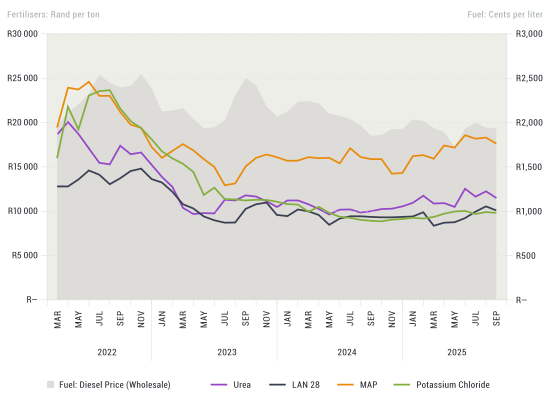
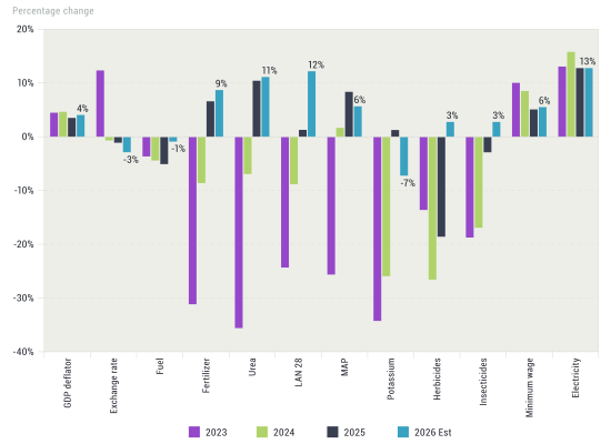
Figure 1.5 presents an overview of the average year-on-year (calendar) percentage changes for key agricultural inputs over the period from 2023 to 2026 (2023 and 2024 are actual changes, and 2025 captures the year to date and the estimated change, while 2026 is an estimated projection). While the GDP inflation was slightly lower in 2025, it is expected to increase again to 4% in 2026. This increase is driven by global economic uncertainty coupled with geopolitical tension, a strong possibility in increased tariffs, as well as domestic increase in electricity cost (13%), minimum wage (6%) and municipal tariffs. Fuel is expected to remain relatively flat.
Herbicide and insecticide costs have seen significant declines over the past three years, and are expected to start increasing again. When comparing the 2025 year to date prices to 2019 average prices, herbicide costs are 6% higher, while insecticide costs are 29% lower. As previously mentioned, fertiliser prices have depicted significant fluctuation over the past few years, but are projected to decline in 2026.
Source: BFAP and Grain SA, October 2025
Methodology, approach and definitions
- A standard operating procedure was used across all crops and regions for generating the cost and income budgets for the 2025/26 production season.
- Deterministic or target yields were based on industry discussions which refers to a yield that should be obtained given a normal production season with normal weather in the respective agro-ecological production regions.
- The farm gate price for each crop was calculated by deducting transport differential, grade differential, handling fees, commission and levies (statutory for seed breeding and technology) from the simulated SAFEX price. For white and yellow maize, industry averages for grade discounts were used to calculate grade differentials.
- The gross production value is then calculated by multiplying the yield with the farm gate price.
- The direct costs are calculated by multiplying the cost per unit by the estimated quantity of input use or application rate.
- For the majority of the crops, it was assumed that own machinery was used, except for speciality operations that is coupled with economies of scale. In such cases, a contracting cost item was allocated. For all crops, provision was made for hail insurance.
- Fertiliser and lime application will vary significantly in regions and across crops, however, an attempt was made to follow a standardised approach across the regions. Micro-elements and foliar feed for selective crops are included in the total fertiliser cost.
- The price for fertiliser nutrients (N, P & K) was calculated by using a weighted approach that accounts for 1. variation in discounts received from suppliers and 2. the time period when fertilisers were purchased.
- Fuel consumption is based on the prevalence production system in each region. The fuel price does not take agricultural rebate into account.
- For plant protection, herbicide, insecticide and fungicides are accounted for based on interaction with industry experts and producers. For instance, in certain regions provision was made for fungicide sprays, but for others where the practise is not common, fungicides were excluded from plant protection costs.
- Repairs and maintenance costs are calculated based on the production system operations.
- For seed, an assumption was made in terms of the majority of crop type area that is cultivated in each region. For instance, the cost of maize seed in Northern-Natal, Mpumalanga and Eastern Free State is based on the assumption that the majority of the area under maize cultivation is yellow maize whereas for the western producing regions, white maize was assumed. An average seed price across various seed companies was used for 1) conventional seeds and 2) GM-technology. The cost of seed per hectare is calculated by multiplying the cost per unit (either kilograms or plant population) by the application rate per hectare. For selective crops, seed treatment was included where relevant. For predominantly oilseeds production, the seed application rate was sub-divided according to own and purchased seed. For own seed use, a cost was also allocated which is based on a realistic crop price (hence, opportunity cost) and seed preparation costs such as sifting and treatment.
- For irrigated crops, the cost of water and electricity was calculated according to typical irrigation application rates at their respective regional costs per millimetre. For instance, variations will occur in the cost for water in areas where predominantly boreholes are used compared to irrigation/water scheme areas.
- The gross margin was calculated by subtracting the direct cost from the gross production value.